Inner Workings of LLMs for Developers - Part 2
Welcome to part 2 of the series on the “Inner Workings of LLMs for Developers”! In Part 1, we took our first crucial step into understanding how machines process language by exploring the classic Bag-of-Words (BoW) model.
We learned how BoW provides a simple yet effective way to convert unstructured text into numerical vectors that a machine can understand. By treating text as an unordered collection of words and simply counting their frequencies, we were able to create a structured representation suitable for tasks like spam filtering and basic document classification. However, we also hit a wall. We discovered that BoW’s simplicity is its biggest limitation. Since it has no concept of word order or semantic meaning, it is blind to the fact that “price” and “cost” are similar, and it can’t tell the difference between “This movie was not good” and “This movie was good, not terrible”.
2013 and 2014
It became clear that plain vector representation of the words was not enough for machines to grasp the most fundamental property of language, words exist in a complex web of relationships. So we needed a methodology to somehow capture their meaning as well as context.
Word Embeddings
If you ask someone which word is more similar to “doctor”—“nurse” or “patient”, most people would say “nurse” makes more sense, since both are medical professionals. But how do we teach a computer that specific relationship, especially when all three words appear together so often? That’s where word embeddings came into the picture.
The conceptual breakthrough that paved the way for word embeddings did not come from computer science, but from linguistics. In the 1950s, linguists such as J.R. Firth and Zellig Harris formulated what is now known as the Distributional Hypothesis. The hypothesis is elegantly summarized by Firth’s famous dictum: “You shall know a word by the company it keeps”. The idea is that the meaning of a word is not an intrinsic property but is defined by the contexts in which it appears. Words that consistently show up in similar linguistic environments are likely to have similar meanings.
While “doctor,” “nurse,” and “patient” all keep company with each other, a machine can analyze millions of sentences and spot subtle patterns.
It might learn that “doctor” and “nurse” often appear in similar contexts like:
- “…consulted with the nurse.” / “…consulted with the doctor.”
- “The doctor’s shift is over.” / “The nurse’s shift is over.”
In contrast, the context for “patient” is consistently different:
- “The doctor treated the patient.” (not “The doctor treated the nurse.”)
- “The patient was admitted by the nurse.”
By recognizing these distinct patterns a computer can deduce that doctors and nurses share a similar role, while a patient’s role is different. This is precisely what a word embedding is designed to capture. It translates these learned relationships into a mathematical form by representing each word as a vector. This vector encodes the word’s meaning in such a way that words with similar contexts, like “doctor” and “nurse,” are positioned closer together in the resulting vector space.
To make this concrete, let’s imagine we have word embeddings for several words like “doctor”, “surgeon”, “nurse”, ”teacher”, “student”, “car” etc. We can represent these embeddings in a table, where each row is a word and each column is a dimension. A dimension is just one piece of information about a word’s meaning, represented by a number. It is simply a feature or a property or an attribute that describes a data point. For example, to describe a car, we could use 3 dimensions/attributes: [speed, price, safety].

As shown in the table, each word is represented by scores across different conceptual dimensions. Words with similar meanings have similar scores. For example, “doctor”, “nurse” and “surgeon” all have high positive scores (e.g., 0.9, 0.8) for the “Medical Pro” dimension, grouping them together. In contrast, a word like “car” scores high on the “Is a Vehicle” dimension but negatively on “Medical Pro,” placing it in a completely different semantic category. This allows a computer to mathematically understand that words with similar vectors are similar in meaning.
💡 Remember in real embeddings, the dimensions don’t have explicit human-readable names like “Medical Pro”, “Is a Location”, as represented in the table. The model learns these dimensions automatically as abstract mathematical properties during the training process. So, a word’s embedding is simply its set of coordinates across hundreds of abstract dimensions (often 300 or more). Each coordinate represents a feature of the word’s meaning that the AI model has learned on its own by analyzing patterns in massive amounts of text.
If we were to plot these embeddings on a 2D graph, we would see that the similar words tend to cluster together.

💡 Sometimes the word embeddings are also referred to as vector embeddings, are they the same? A vector embedding is a broader term used in AI to represent any entity (like a word, a user, a sentence or an image) as a numeric vector whereas word embeddings are just one specific type of vector embedding, specialized for representing the meaning of words.
Now that we understand what word embeddings are, the question is how do we generate them? This is where Word2Vec comes into the picture.
Word2Vec
Word2Vec (short for Word to Vector) introduced by a team of researchers at Google in 2013, was the first successful technique of converting words to vectors, thereby capturing their meaning and relationship with surrounding text in the form of word embeddings.
In order for the model to start generating word embeddings, it must first be trained on enormous amounts of text data like a library of books, blogs, articles, Wikipedia etc. By analyzing which words frequently appear near each other, it starts to learn patterns about the language. But before the model can learn, the raw text must be turned into a structured dataset suitable for training. Word2Vec accomplishes this by using a “sliding window” approach. A window of a fixed size moves across the text and at each position, it generates one or more training dataset samples.

Let’s understand this with an example. Consider the sentence: “The nurse assisted the doctor with the patient’s treatment at the hospital.” Suppose this sentence is part of a larger training corpus. We’ll use it to walk through how the Word2Vec model generates training samples and eventually learns useful word embeddings.
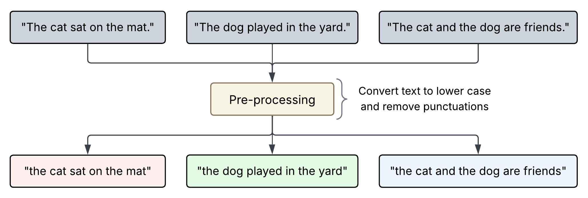
Step 1: Pre-processing
Just like BoW, the first step is to clean the training data to reduce the complexity of the vocabulary and allow the model to focus on learning meaningful semantic signals.

💡 In this example, the vocabulary size comes out to be 9, however in reality it can be thousands or even millions. The vocabulary isn’t built from a single sentence but from a massive collection of text (a “corpus”) like all of Wikipedia or a large portion of the internet.
Step 2: Creating training dataset
With the corpus transformed into a clean sequence of tokens, the next stage involves extracting training instances. For this, Word2Vec proposes two primary architectures:
- Continuous Bag-of-Words (CBOW)
- Skip-gram Let’s understand each of these architectures in detail.
Continuous Bag-of-Words (CBOW)
The CBOW architecture operates on the principle of predicting the target word based on its surrounding context words. It essentially asks the question: “Given these surrounding words, what is the most likely word to be in the middle?” The context words are treated as a “bag” of words, meaning their order is not considered in the standard implementation. This process primarily relies on a “sliding window” technique. This technique systematically moves through the token sequence to define a “local context” for each word.

In the above example, a window size of 2 means that for any given word, we consider up to two words to its left and up to two words to its right as its context. The total potential size of the context for any given word is therefore four.
Let’s apply CBOW to the tokenized output from Step 1 ['the', 'nurse', 'assisted', 'the', 'doctor', 'with', 'the', 'patient', 'treatment', 'at', 'the', 'hospital'] considering a sliding window size of 2 to obtain a training dataset.
Iteration 1:
For the first iteration, the context words are “nurse” and “assisted” (window size 2), and the target word is “the”. Since there are no words before the first “the”, we only take the two words that come after it.

Iteration 2:
The next context words are “the” (left boundary) and “assisted”, “the” (right boundary) and target word is “nurse”.

Iteration 3:
Context words are “the”, “nurse” (left boundary) and “the”, “doctor” (right boundary) and the target word is “assisted”.

We continue to iterate over the tokenized input until we reach the end of the input data. The final training dataset would look as below:

Skip-gram
The Skip-gram architecture works in the opposite direction. Instead of using the context to predict the target, it uses the target word to predict its surrounding context words. It asks, “Given this central word, what are the words likely to be found in its vicinity?” This approach generates more training samples for the same window position.

Let’s apply Skip-gram to the tokenized output from Step 1 ['the', 'nurse', 'assisted', 'the', 'doctor', 'with', 'the', 'patient', 'treatment', 'at', 'the', 'hospital'] considering a sliding window size of 2 to obtain a training dataset.
Iteration 1:
For the first iteration, the target word (i.e. input word) is “the”. Since the size of the sliding window is 2, the model creates two training samples, one for each context word - “nurse”, “assisted”. For the first word in the sentence, the sliding window can only look forward, not backward.

Iteration 2:
For the next iteration, the target word shifts to “nurse”. This time we have one context word - “the”, on the left boundary of the target word and two context words - “assisted” and “the”, on the right boundary of the target word so the model creates a total of three training samples.

Iteration 3:
The target word is “assisted” with two context words on each side so the model creates a total of four training samples.

Skip-gram continues to iterate over the input until it reaches the end of the sentence. The final training dataset would look like below:

With Skip-gram, you will notice that it produces a higher number of training samples as compared to CBOW.
Step 3: Training Process
The Word2Vec model, at its core, is a simple neural network that learns by manipulating two key matrices:
- Embedding Matrix
- Context Matrix Let’s understand the two matrices in detail.
Embedding Matrix (E)
The Embedding Matrix is the primary data structure where the final word embeddings of a trained model are stored. Let’s understand the structure of this matrix.

Each row of this matrix corresponds to a word in our vocabulary (obtained in Step 1) and holds its vector representation. The columns are represented by dimensions or attributes, which are abstract mathematical properties that represent relationships between words. Initially, since the model is untrained, this matrix is populated with random numbers because the model lacks any prior knowledge of word relationships.
During the training process, this matrix is used to lookup the vector for the input words.
Context Matrix (C)
The Context Matrix is used for generating predictions during the training process. It also contains the vector for every word in the vocabulary. However, its structure is different from the Embedding Matrix.

Each row in the Context Matrix represents the same dimensions (d) as in the embedding matrix while each word in the vocabulary (v) is represented in columns. Similar to the embedding matrix, the context matrix is also initialized with random numbers at the start of the training process.
During the training process (which we’ll look at next), the interaction between a row from Embedding Matrix (representing an input word) and a column from Context Matrix (representing a potential output word) generates a score that indicates how likely that pair is to appear together.
Next, let’s understand the training process for Word2Vec using the Skip-gram training dataset as an example:
Let’s take the first sample from the training dataset and pass it to the model:

The model’s task is to take the word “the” and predict its likely neighbor.
Step 1: Lookup Vector
The model retrieves the current vectors for the input word “the” from the Embedding Matrix (E): E[“the”] = [0.182, -0.463, 0.771, -0.023, …, …, 0.314]
Step 2: Score and Predict
This step predicts the most likely neighbor for the input word “the” by asking a simple question: ‘How similar is “the” to every other word in our vocabulary?’
To find the answer, the model takes the input word’s vector and compares it against every column in the Context Matrix using mathematical operations like dot product and Softmax to come up with a list of probabilities showing how likely each word is to be the correct neighbor. Its final probabilities would looks something like this:

The model assigns highest probability to the word “hospital” as the most likely neighbor of the input word “the”. This is an incorrect prediction since we know from the sample dataset (i.e. the ground truth) the correct prediction should be the word “nurse”. This is expected at this stage since this is an untrained model.
💡 As you may have noticed above, the model calculates the probability scores for all the words in the vocabulary. Imagine if the size of the vocabulary is 50k, 500k or in millions, performing this calculation for every single input word would become a computational bottleneck, making the training process incredibly slow and inefficient. Clearly, a smarter way is needed to train the model. More on this later.
Step 3: Calculate Error
In this step, the model’s prediction is compared to the actual output word from the training pair to calculate the error vector. The error is the gap between what the model predicted and what it should have predicted. The model gave “hospital” a very high score and the correct word, “nurse” a very low score. This error signal tells us exactly how to update the numbers in our matrices to make the correct prediction more likely next time.
Step 4: Update
This step represents the learning aspect of the training process. The model learns by adjusting its embeddings based on the error found in the previous step.
It makes the following adjustments to the Context Matrix (C):
- The output vector for the correct word,
C["nurse"], is nudged to become more similar to the input vectorE["the"]. - Every other column in the Context Matrix (
C["hospital"],C["assisted"],C["car"], etc.) is nudged to become less similar to the input vectorE["the"].
Additionally, the following adjustment is made to the Embedding Matrix (E):
The vector E["the"] is updated to become more similar to C["nurse"] while also being pushed away from all other vectors, with the strongest push coming from C["hospital"].
This completes a single training step. The Embedding Matrix is updated for the input word based on the prediction error. The Context Matrix guides this adjustment, drawing the input vector closer to the correct target word and further from incorrect ones. Consequently, the Embedding Matrix becomes slightly smarter than before. By repeating this process millions of times, the Embedding Matrix develops into a robust and precise language representation.
But what about the problem of computational bottleneck?
In the steps above, I mentioned that the model calculates a probability score for every single word in the vocabulary. Imagine a vocabulary with 50,000 words and 300 dimensions. For every single training sample, the model would have to:
- Calculate 50,000 individual scores.
- Update 15 million weights (50,000 x 300) in the Context Matrix based on those scores.
This is a massive computational bottleneck that makes training on large datasets prohibitively slow.
The Solution: Reframe the problem statement with Negative Sampling
Instead of asking a huge multi-choice question (“Which of these 50,000 words is the correct one?”), negative sampling changes the task to a much simpler Yes or No question:
“For this given pair of words, are they actually neighbors or not?”
This is a brilliant simplification. Instead of one giant, slow calculation, we do several tiny, fast ones.
So, let’s understand how Negative Sampling works.
Step 1: Select the Positive Sample
First, we take our ground truth pair. This is our “positive” example, the one we want the model to learn is correct. We give it a label of 1.

Step 2: Add Negative Samples
Next, we pick random “negative” or “noise” words from the vocabulary. These are the words that we know are not the neighbors of the input word and we give them a label of 0.

Step 3: Score and Predict
This step is now transformed. Instead of doing a massive number of calculations for every single input word, we have a small, manageable task with just 4 samples (1 positive + 3 negative). The model calculates the probability scores for only these 4 samples.
Since the model is untrained, its predictions are essentially random. For example, it might predict “phone” as a neighbor for the input word “the”. The model then compares this output to the correct label, and the resulting mismatch is used to calculate an error and drive the learning process.
Step 4: Update
The update (or learning) is now extremely efficient and targeted.
- Positive Update: The input vector
E["the"]and the output vectorC["nurse"]are nudged closer together, to increase their similarity score. - Negative Updates: The input vector
E["the"]is nudged away from the output vectors for our three negative samples:C["phone"],C["hospital"]andC["art"].
This optimization is what makes training Word2Vec on massive vocabularies feasible.
Repeating this process multiple times pulls the vectors for related words like “doctor” and “nurse” closer together, while pushing unrelated words like “car” and “phone” further apart. The final result of this training process is the Embedding Matrix that serves as a powerful knowledge base that captures the words’ underlying meaning, context, and semantic relationship, serving as a foundational building block for nearly all modern Natural Language Processing (NLP) tasks.
Challenges with Word2Vec
The Polysemy Problem: One word, many meanings
The biggest challenge for Word2Vec is that it generates one single, static vector for each unique word in its vocabulary. This vector is created during training by averaging all the different contexts in which the word appeared.
In our example, the model was trained on the sentence: “The nurse assisted the doctor with the patient’s treatment at the hospital.” During the training process, the only context the model ever saw for the word “doctor” was purely medical. It appeared alongside words like: nurse, assisted, patient, treatment and hospital. Because of this, the training process created exactly one vector for the word “doctor” which is very close to the vectors for other medical terms.
Now, let’s give our trained model a new sentence that uses the word “doctor” in a completely different sense:
“She is a doctor of philosophy, and her thesis on ancient Rome was brilliant.”
In this sentence, “doctor” refers to a Ph.D., an academic who holds the highest university degree. The true semantic neighbors of “doctor” in this context are words like professor, university, thesis, academic, and history.
When the model processes this new sentence, it looks up the word “doctor” in its Embedding Matrix. It has no choice but to retrieve the one and only vector it has, the one that represents a medical doctor. The model is trying to understand a sentence about academic achievement using a vector that represents medical practice. This is a fundamental mismatch. It has no mechanism to adapt the meaning of “doctor” based on the surrounding words like “philosophy” or “thesis.” This inability to distinguish between different senses of a word is the essence of the problem.
Blind to Order and Syntax
A second, equally critical flaw of static, window-based models like Word2Vec is their general disregard for word order and syntax. Word2Vec’s training process uses a context window, treating the words surrounding a target word as a “bag of words”. While it learns which words appear near each other, it does not effectively encode the grammatical structure or the precise positional relationships between them.
The classic example “Man bites dog” versus “Dog bites man” illustrates this perfectly. Both sentences contain the exact same words, and in a small context window, the co-occurrence patterns are identical. A model like Word2Vec would see “dog,” “bites,” and “man” in close proximity in both cases and would struggle to distinguish the profound difference in meaning. This inability to capture how meaning is constructed from the arrangement of words, is a severe limitation for any task that requires more than a surface-level understanding of text.
So, how do we create word embeddings that are not static, but dynamic and context-aware?
We’ll answer that question in Part 3.

Leave a comment